How to Use Python to Parse & Pivot Server Log Files for SEO

Search engine crawl data found within log files is a fantastic source of information for any SEO professional.

By analyzing log files, you can gain an understanding of exactly how search engines are crawling and interpreting your website – clarity you simply cannot get when relying upon third-party tools.

This will allow you to:

• Validate your theories by providing indisputable evidence of how search engines are behaving.
• Prioritize your findings by helping you to understand the scale of a problem and the likely impact of fixing it.
• Uncover additional issues that aren’t visible when using other data sources.

But despite the multitude of benefits, log file data isn’t used as frequently as it should be. The reasons are understandable:

• Accessing the data usually involves going through a dev team, which can take time.
• The raw files can be huge and provided in an unfriendly format, so parsing the data takes effort.
• Tools designed to make the process easier may need to be integrated before the data can be piped to it, and the costs can be prohibitive.

All of these issues are perfectly valid barriers to entry, but they don’t have to be insurmountable.

With a bit of basic coding knowledge, you can automate the entire process. That’s exactly what we’re going to do in this step-by-step lesson on using Python to analyze server logs for SEO.

You’ll find a script to get you started, too.

Initial Considerations

One of the biggest challenges in parsing log file data is the sheer number of potential formats. Apache, Nginx, and IIS offer a range of different options and allow users to customize the data points returned.

To complicate matters further, many websites now use CDN providers like Cloudflare, Cloudfront, and Akamai to serve up content from the closest edge location to a user. Each of these has its own formats, as well.

We’ll focus on the Combined Log Format for this post, as this is the default for Nginx and a common choice on Apache servers.

If you’re unsure what type of format you’re dealing with, services like Builtwith and Wappalyzer both provide excellent information about a website’s tech stack. They can help you determine this if you don’t have direct access to a technical stakeholder.

Still none the wiser? Try opening one of the raw files.

Often, comments are provided with information on the specific fields, which can then be cross-referenced.

#Fields: time c-ip cs-method cs-uri-stem sc-status cs-version 
17:42:15 172.16.255.255 GET /default.htm 200 HTTP/1.0

Another consideration is what search engines we want to include, as this will need to be factored into our initial filtering and validation.

To simplify things, we’ll focus on Google, given its dominant 88% US market share.

Let’s get started.

1. Identify Files and Determining Formats

To perform meaningful SEO analysis, we want a minimum of ~100k requests and 2-4 weeks’ worth of data for the average site.

Due to the file sizes involved, logs are usually split into individual days. It’s virtually guaranteed that you’ll receive multiple files to process.

As we don’t know how many files we’ll be dealing with unless we combine them before running the script, an important first step is to generate a list of all of the files in our folder using the glob module.

This allows us to return any file matching a pattern that we specify. As an example, the following code would match any TXT file.

import glob

files = glob.glob('*.txt')

Log files can be provided in a variety of file formats, however, not just TXT.

In fact, at times the file extension may not be one you recognize. Here’s a raw log file from Akamai’s Log Delivery Service, which illustrates this perfectly:

bot_log_100011.esw3c_waf_S.202160250000-2000-41

Additionally, it’s possible that the files received are split across multiple subfolders, and we don’t want to waste time copying these into a singular location.

Thankfully, glob supports both recursive searches and wildcard operators. This means that we can generate a list of all the files within a subfolder or child subfolders.

files = glob.glob('**/*.*', recursive=True)

Next, we want to identify what types of files are within our list. To do this, the MIME type of the specific file can be detected. This will tell us exactly what type of file we’re dealing with, regardless of the extension.

This can be achieved using python-magic, a wrapper around the libmagic C library, and creating a simple function.

pip install python-magic
pip install libmagic

import magic

def file_type(file_path):
    mime = magic.from_file(file_path, mime=True)
    return mime

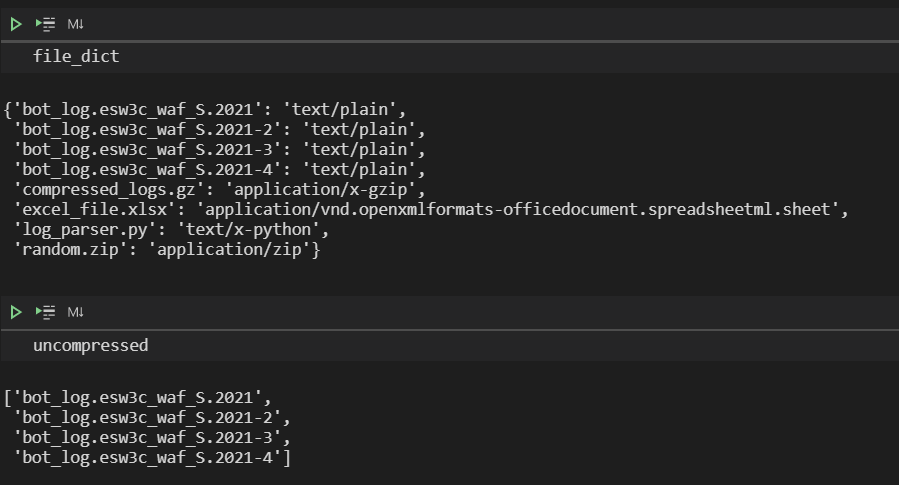
List comprehension can then be used to loop through our files and apply the function, creating a dictionary to store both the names and types.

file_types = [file_type(file) for file in files]

file_dict = dict(zip(files, file_types))

Finally, a function and a while loop to extract a list of files that return a MIME type of text/plain and exclude anything else.

uncompressed = []

def file_identifier(file):
    for key, value in file_dict.items():
        if file in value:
            uncompressed.append(key)

while file_identifier('text/plain'):
    file_identifier('text/plain') in file_dict

2. Extract Search Engine Requests

After filtering down the files in our folder(s), the next step is to filter the files themselves by only extracting the requests that we care about.

This removes the need to combine the files using command-line utilities like GREP or FINDSTR, saving an inevitable 5-10 minute search through open notebook tabs and bookmarks to find the correct command.

In this instance, as we only want Googlebot requests, searching for ‘Googlebot’ will match all of the relevant user agents.

We can use Python’s open function to read and write our file and Python’s regex module, RE, to perform the search.

import re

pattern = 'Googlebot'
new_file = open('./googlebot.txt', 'w', encoding='utf8')

for txt_files in uncompressed:
    with open(txt_files, 'r', encoding='utf8') as text_file:
        for line in text_file:
            if re.search(pattern, line):
                new_file.write(line)

Regex makes this easily scalable using an OR operator.

pattern = 'Googlebot|bingbot'

3. Parse Requests

In a previous post, Hamlet Batista provided guidance on how to use regex to parse requests.

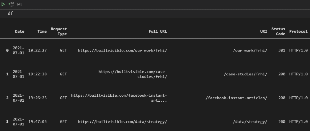
As an alternative approach, we’ll be using Pandas‘ powerful inbuilt CSV parser and some basic data processing functions to:

1. Drop unnecessary columns.
2. Format the timestamp.
3. Create a column with full URLs.
4. Rename and reorder the remaining columns.

Rather than hardcoding a domain name, the input function can be used to prompt the user and save this as a variable.

whole_url = input('Please enter full domain with protocol: ') # get domain from user input

df = pd.read_csv('./googlebot.txt', sep='\s+', error_bad_lines=False, header=None, low_memory=False) # import logs

df.drop([1, 2, 4], axis=1, inplace=True) # drop unwanted columns/characters

df[3] = df[3].str.replace('[', '') # split time stamp into two
df[['Date', 'Time']] = df[3].str.split(':', 1, expand=True)

df[['Request Type', 'URI', 'Protocol']] = df[5].str.split(' ', 2, expand=True) # split uri request into columns
df.drop([3, 5], axis=1, inplace=True)

df.rename(columns = {0:'IP', 6:'Status Code', 7:'Bytes', 8:'Referrer URL', 9:'User Agent'}, inplace=True) #rename columns

df['Full URL'] = whole_url + df['URI'] # concatenate domain name

df['Date'] = pd.to_datetime(df['Date']) # declare data types
df[['Status Code', 'Bytes']] = df[['Status Code', 'Bytes']].apply(pd.to_numeric)

df = df[['Date', 'Time', 'Request Type', 'Full URL', 'URI', 'Status Code', 'Protocol', 'Referrer URL', 'Bytes', 'User Agent', 'IP']] # reorder columns

4. Validate Requests

It’s incredibly easy to spoof search engine user agents, making request validation a vital part of the process, lest we end up drawing false conclusions by analyzing our own third-party crawls.

To do this, we’re going to install a library called dnspython and perform a reverse DNS.

Pandas can be used to drop duplicate IPs and run the lookups on this smaller DataFrame, before reapplying the results and filtering out any invalid requests.

from dns import resolver, reversename
def reverseDns(ip):
    try:
        return str(resolver.query(reversename.from_address(ip), 'PTR')[0])
    except:
        return 'N/A'

logs_filtered = df.drop_duplicates(['IP']).copy() # create DF with dupliate ips filtered for check

logs_filtered['DNS'] = logs_filtered['IP'].apply(reverseDns)  # create DNS column with the reverse IP DNS result

logs_filtered = df.merge(logs_filtered[['IP', 'DNS']], how='left', on=['IP'])  # merge DNS column to full logs matching IP

logs_filtered = logs_filtered[logs_filtered['DNS'].str.contains('googlebot.com')]  # filter to verified Googlebot

logs_filtered.drop(['IP', 'DNS'], axis=1, inplace=True)  # drop dns/ip columns

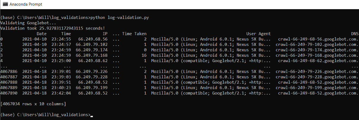
Taking this approach will drastically speed up the lookups, validating millions of requests in minutes.

In the example below, ~4 million rows of requests were processed in 26 seconds.

5. Pivot the Data

After validation, we’re left with a cleansed, well-formatted data set and can begin pivoting this data to more easily analyze data points of interest.

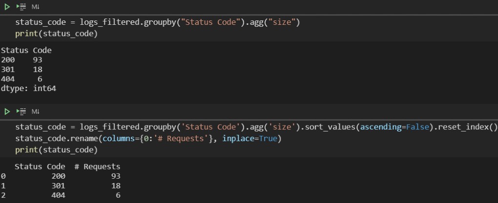
First off, let’s begin with some simple aggregation using Pandas’ groupby and agg functions to perform a count of the number of requests for different status codes.

status_code = logs_filtered.groupby('Status Code').agg('size')

To replicate the type of count you are used to in Excel, it’s worth noting that we need to specify an aggregate function of ‘size’, not ‘count’.

Using count will invoke the function on all columns within the DataFrame, and null values are handled differently.

Resetting the index will restore the headers for both columns, and the latter column can be renamed to something more meaningful.

status_code = logs_filtered.groupby('Status Code').agg('size').sort_values(ascending=False).reset_index()

status_code.rename(columns={0:'# Requests'}, inplace=True)

For more advanced data manipulation, Pandas’ inbuilt pivot tables offer functionality comparable to Excel, making complex aggregations possible with a singular line of code.

At its most basic level, the function requires a specified DataFrame and index – or indexes if a multi-index is required – and returns the corresponding values.

pd.pivot_table(logs_filtered, index['Full URL'])

For greater specificity, the required values can be declared and aggregations – sum, mean, etc – applied using the aggfunc parameter.

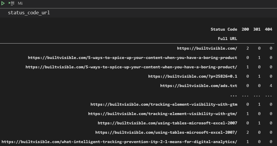
Also worth mentioning is the columns parameter, which allows us to display values horizontally for clearer output.

status_code_url = pd.pivot_table(logs_filtered, index=['Full URL'], columns=['Status Code'], aggfunc='size', fill_value=0)

Here’s a slightly more complex example, which provides a count of the unique URLs crawled per user agent per day, rather than just a count of the number of requests.

user_agent_url = pd.pivot_table(logs_filtered, index=['User Agent'], values=['Full URL'], columns=['Date'], aggfunc=pd.Series.nunique, fill_value=0)

If you’re still struggling with the syntax, check out Mito. It allows you to interact with a visual interface within Jupyter when using JupyterLab, but still outputs the relevant code.

Incorporating Ranges

For data points like bytes which are likely to have many different numerical values, it makes sense to bucket the data.

To do so, we can define our intervals within a list and then use the cut function to sort the values into bins, specifying np.inf to catch anything above the maximum value declared.

byte_range = [0, 50000, 100000, 200000, 500000, 1000000, np.inf]

bytes_grouped_ranges = (logs_filtered.groupby(pd.cut(logs_filtered['Bytes'], bins=byte_range, precision=0))
    .agg('size')
    .reset_index()
)

bytes_grouped_ranges.rename(columns={0: '# Requests'}, inplace=True)

Interval notation is used within the output to define exact ranges, e.g.

(50000 100000]

The round brackets indicate when a number is not included and a square bracket when it is included. So, in the above example, the bucket contains data points with a value of between 50,001 and 100,000.

6. Export

The final step in our process is to export our log data and pivots.

For ease of analysis, it makes sense to export this to an Excel file (XLSX) rather than a CSV. XLSX files support multiple sheets, which means that all the DataFrames can be combined in the same file.

This can be achieved using to excel. In this case, an ExcelWriter object also needs to be specified because more than one sheet is being added into the same workbook.

writer = pd.ExcelWriter('logs_export.xlsx', engine='xlsxwriter', datetime_format='dd/mm/yyyy', options={'strings_to_urls': False})

logs_filtered.to_excel(writer, sheet_name='Master', index=False)
pivot1.to_excel(writer, sheet_name='My pivot')

writer.save()

When exporting a large number of pivots, it helps to simplify things by storing DataFrames and sheet names in a dictionary and using a for loop.

sheet_names = {
    'Request Status Codes Per Day': status_code_date,
    'URL Status Codes': status_code_url,
    'User Agent Requests Per Day': user_agent_date,
    'User Agent Requests Unique URLs': user_agent_url,
    }

for sheet, name in sheet_names.items():
    name.to_excel(writer, sheet_name=sheet)

One last complication is that Excel has a row limit of 1,048,576. We’re exporting every request, so this could cause problems when dealing with large samples.

Because CSV files have no limit, an if statement can be employed to add in a CSV export as a fallback.

If the length of the log file DataFrame is greater than 1,048,576, this will instead be exported as a CSV, preventing the script from failing while still combining the pivots into a singular export.

if len(logs_filtered) <= 1048576:
    logs_filtered.to_excel(writer, sheet_name='Master', index=False)
else:
    logs_filtered.to_csv('./logs_export.csv', index=False)

Final Thoughts

The additional insights that can be gleaned from log file data are well worth investing some time in.

If you’ve been avoiding leveraging this data due to the complexities involved, my hope is that this post will convince you that these can be overcome.

For those with access to tools already who are interested in coding, I hope breaking down this process end-to-end has given you a greater understanding of the considerations involved when creating a larger script to automate repetitive, time-consuming tasks.

The full script I created can be found here on Github.

This includes additional extras such as GSC API integration, more pivots, and support for two more log formats: Amazon ELB and W3C (used by IIS).

To add in another format, include the name within the log_fomats list on line 17 and add an additional elif statement on line 193 (or edit one of the existing ones).

There is, of course, massive scope to expand this further. Stay tuned for a part two post that will cover the incorporation of data from third-party crawlers, more advanced pivots, and data visualization.

More Resources:

• How to Use Python to Analyze SEO Data: A Reference Guide
• 8 Python Libraries for SEO & How To Use Them
• Advanced Technical SEO: A Complete Guide

Image Credits

All screenshots taken by author, July 2021