How to Use Python to Forecast Demand, Traffic & More for SEO

Whether it’s search demand, revenue, or traffic from organic search, at some point in your SEO career, you’re bound to be asked to deliver a forecast.

In this column, you’ll learn how to do just that accurately and efficiently, thanks to Python.

We’re going to explore how to:

• Pull and plot your data.
• Use automated methods to estimate the best fit model parameters.
• Apply the Augmented Dickey-Fuller method (ADF) to statistically test a time series.
• Estimate the number of parameters for a SARIMA model.
• Test your models and begin making forecasts.
• Interpret and export your forecasts.

Before we get into it, let’s define the data. Regardless of the type of metric, we’re attempting to forecast, that data happens over time.

In most cases, this is likely to be over a series of dates. So effectively, the techniques we’re disclosing here are time series forecasting techniques.

So Why Forecast?

To answer a question with a question, why wouldn’t you forecast?

These techniques have been long used in finance for stock prices, for example, and in other fields. Why should SEO be any different?

With multiple interests such as the budget holder and other colleagues – say, the SEO manager and marketing director – there will be expectations as to what the organic search channel can deliver and whether those expectations will be met, or not.

Forecasts provide a data-driven answer.

Helpful Forecasting Info for SEO Pros

Taking the data-driven approach using Python, there are a few things to bear in mind:

Forecasts work best when there is a lot of historical data.

The cadence of the data will determine the time frame needed for your forecast.

For example, if you have daily data like you would in your website analytics then you’ll have over 720 data points, which are fine.

With Google Trends, which has a weekly cadence, you’ll need at least 5 years to get 250 data points.

In any case, you should aim for a timeframe that gives you at least 200 data points (a number plucked from my personal experience).

Models like consistency.

If your data trend has a pattern — for example, it’s cyclical because there is seasonality — then your forecasts are more likely to be reliable.

For that reason, forecasts don’t handle breakout trends very well because there’s no historical data to base the future on, as we’ll see later.

So how do forecasting models work? There are a few aspects the models will address about the time series data:

Autocorrelation

Autocorrelation is the extent to which the data point is similar to the data point that came before it.

This can give the model information as to how much impact an event in time has over the search traffic and whether the pattern is seasonal.

Seasonality

Seasonality informs the model as to whether there is a cyclical pattern, and the properties of the pattern, e.g.: how long, or the size of the variation between the highs and lows.

Stationarity

Stationarity is the measure of how the overall trend is changing over time. A non-stationary trend would show a general trend up or down, despite the highs and lows of the seasonal cycles.

With the above in mind, models will “do” things to the data to make it more of a straight line and therefore more predictable.

With the whistlestop theory out of the way, let’s start forecasting.

Exploring Your Data

# Import your libraries
import pandas as pd
from statsmodels.tsa.statespace.sarimax import SARIMAX
from statsmodels.graphics.tsaplots import plot_acf, plot_pacf 
from statsmodels.tsa.seasonal import seasonal_decompose                        
from sklearn.metrics import mean_squared_error
from statsmodels.tools.eval_measures import rmse
import warnings
warnings.filterwarnings("ignore")
from pmdarima import auto_arima

We’re using Google Trends data, which is a CSV export.

These techniques can be used on any time series data, be it your own, your client’s or company’s clicks, revenues, etc.

# Import Google Trends Data
df = pd.read_csv("exports/keyword_gtrends_df.csv", index_col=0)
df.head()

Screenshot from Google Trends, September 2021

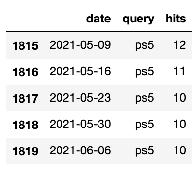
As we’d expect, the data from Google Trends is a very simple time series with date, query, and hits spanning a 5-year period.

It’s time to format the dataframe to go from long to wide.

This allows us to see the data with each search query as columns:

df_unstacked = ps_trends.set_index(["date", "query"]).unstack(level=-1)
df_unstacked.columns.set_names(['hits', 'query'], inplace=True)
ps_unstacked = df_unstacked.droplevel('hits', axis=1)
ps_unstacked.columns = [c.replace(' ', '_') for c in ps_unstacked.columns]
ps_unstacked = ps_unstacked.reset_index()
ps_unstacked.head()

Screenshot from Google Trends, September 2021

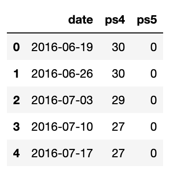
We no longer have a hits column, as these are the values of the queries in their respective columns.

This format is not only useful for SARIMA (which we will be exploring here) but also for neural networks such as Long short-term memory (LSTM).

Let’s plot the data:

ps_unstacked.plot(figsize=(10,5))

Screenshot from Google Trends, September 2021

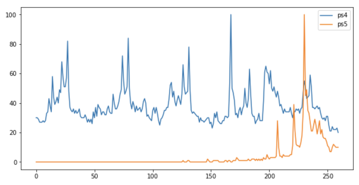
From the plot (above), you’ll note that the profiles of “PS4” and “PS5” are both different. For the non-gamers among you, “PS4” is the 4th generation of the Sony Playstation console, and “PS5” the fifth.

“PS4” searches are highly seasonal as they’re an established product and have a regular pattern apart from the end when the “PS5” emerges.

The “PS5” didn’t exist 5 years ago, which would explain the absence of a trend in the first 4 years of the plot above.

I’ve chosen those two queries to help illustrate the difference in forecasting effectiveness for the two very different characteristics.

Decomposing the Trend

Let’s now decompose the seasonal (or non-seasonal) characteristics of each trend:

ps_unstacked.set_index("date", inplace=True)
ps_unstacked.index = pd.to_datetime(ps_unstacked.index)

query_col = 'ps5'

a = seasonal_decompose(ps_unstacked[query_col], model = "add")
a.plot();

Screenshot from Google Trends, September 2021

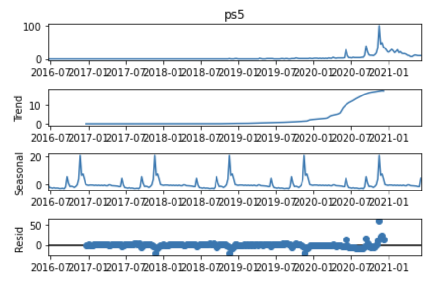
The above shows the time series data and the overall smoothed trend arising from 2020.

The seasonal trend box shows repeated peaks, which indicates that there is seasonality from 2016. However, it doesn’t seem particularly reliable given how flat the time series is from 2016 until 2020.

Also suspicious is the lack of noise, as the seasonal plot shows a virtually uniform pattern repeating periodically.

The Resid (which stands for “Residual”) shows any pattern of what’s left of the time series data after accounting for seasonality and trend, which in effect is nothing until 2020 as it’s at zero most of the time.

For “ps4”:

Screenshot from Google Trends, September 2021

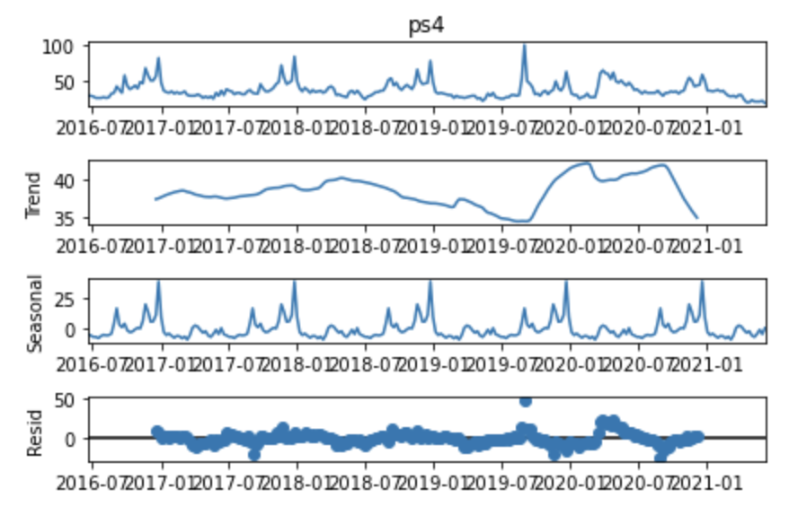
We can see fluctuation over the short term (Seasonality) and long term (Trend), with some noise (Resid).

The next step is to use the Augmented Dickey-Fuller method (ADF) to statistically test whether a given Time series is stationary or not.

from pmdarima.arima import ADFTest

adf_test = ADFTest(alpha=0.05)
adf_test.should_diff(ps_unstacked[query_col])
PS4: (0.09760939899434763, True)
PS5: (0.01, False)

We can see the p-value of “PS5” shown above is more than 0.05, which means that the time series data is not stationary and therefore needs differencing.

“PS4,” on the other hand, is less than 0.05 at 0.01; it’s stationary and doesn’t require differencing.

The point of all of this is to understand the parameters that would be used if we were manually building a model to forecast Google searches.

Fitting Your SARIMA Model

Since we’ll be using automated methods to estimate the best fit model parameters (later), we’re now going to estimate the number of parameters for our SARIMA model.

I’ve chosen SARIMA because it’s easy to install. Although Facebook’s Prophet is elegant mathematically speaking (it uses Monte Carlo methods), it’s not maintained enough and many users may have problems trying to install it.

In any case, SARIMA compares quite well to Prophet in terms of accuracy.

To estimate the parameters for our SARIMA model, note that we set m to 52 as there are 52 weeks in a year, which is how the periods are spaced in Google Trends.

We also set all of the parameters to start at 0 so that we can let the auto_arima do the heavy lifting and search for the values that best fit the data for forecasting.

ps5_s = auto_arima(ps_unstacked['ps4'],
           trace=True,
           m=52, # there are 52 periods per season (weekly data)
           start_p=0,
           start_d=0,
           start_q=0, 
           seasonal=False)

Response to above:

Performing stepwise search to minimize aic

 ARIMA(3,0,3)(0,0,0)[0]             : AIC=1842.301, Time=0.26 sec
 ARIMA(0,0,0)(0,0,0)[0]             : AIC=2651.089, Time=0.01 sec
...
 ARIMA(5,0,4)(0,0,0)[0] intercept   : AIC=1829.109, Time=0.51 sec

Best model:  ARIMA(4,0,3)(0,0,0)[0] intercept
Total fit time: 6.601 seconds

The printout above shows that the parameters that get the best results are:

PS4: ARIMA(4,0,3)(0,0,0)
PS5: ARIMA(3,1,3)(0,0,0)

The PS5 estimate is further detailed when printing out the model summary:

ps5_s.summary()

Screenshot from SARIMA, September 2021

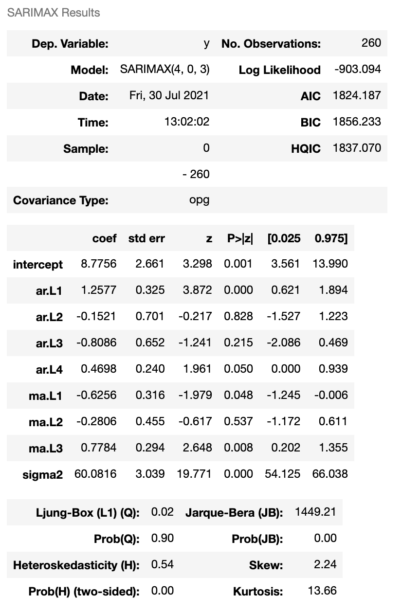
What’s happening is this: The function is looking to minimize the probability of error measured by both the Akaike’s Information Criterion (AIC) and Bayesian Information Criterion.

AIC = -2Log(L) + 2(p + q + k + 1)

Such that L is the likelihood of the data, k = 1 if c ≠ 0 and k = 0 if c = 0

BIC = AIC + [log(T) - 2] + (p + q + k + 1)

By minimizing AIC and BIC, we get the best-estimated parameters for p and q.

Test the Model

Now that we have the parameters, we can begin making forecasts. First, we’re going to see how the model performs over past data. This gives us some indication as to how well the model could perform for future periods.

ps4_order = ps4_s.get_params()['order']
ps4_seasorder = ps4_s.get_params()['seasonal_order']
ps5_order = ps5_s.get_params()['order']
ps5_seasorder = ps5_s.get_params()['seasonal_order']

params = {
    "ps4": {"order": ps4_order, "seasonal_order": ps4_seasorder},
    "ps5": {"order": ps5_order, "seasonal_order": ps5_seasorder}
}

results = []
fig, axs = plt.subplots(len(X.columns), 1, figsize=(24, 12))  

for i, col in enumerate(X.columns):
    #Fit best model for each column
    arima_model = SARIMAX(train_data[col],
                          order = params[col]["order"],
                          seasonal_order = params[col]["seasonal_order"])
    arima_result = arima_model.fit()

    #Predict
    arima_pred = arima_result.predict(start = len(train_data),
                                      end = len(X)-1, typ="levels")\
                             .rename("ARIMA Predictions")

    #Plot predictions
    test_data[col].plot(figsize = (8,4), legend=True, ax=axs[i])
    arima_pred.plot(legend = True, ax=axs[i])
    arima_rmse_error = rmse(test_data[col], arima_pred)

    mean_value = X[col].mean()
    results.append((col, arima_pred, arima_rmse_error, mean_value))
    print(f'Column: {col} --> RMSE Error: {arima_rmse_error} - Mean: {mean_value}\n')

Column: ps4 --> RMSE Error: 8.626764032898576 - Mean: 37.83461538461538
Column: ps5 --> RMSE Error: 27.552818032476257 - Mean: 3.973076923076923

The forecasts show the models are good when there is enough history until they suddenly change, as they have for PS4 from March onwards.

For PS5, the models are hopeless virtually from the get-go.

We know this because the Root Mean Squared Error (RMSE) is 8.62 for PS4, which is more than a third of the PS5 RMSE of 27.5. Given that Google Trends varies from 0 to 100, this is a 27% margin of error.

Forecast the Future

At this point, we’ll now make the foolhardy attempt to forecast the future based on the data we have to date:

oos_train_data = ps_unstacked
oos_train_data.tail()

Screenshot from Google Trends, September 2021

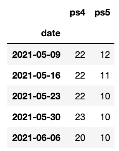
As you can see from the table extract above, we’re now using all available data.

Now, we shall predict the next 6 months (defined as 26 weeks) in the code below:

oos_results = []
weeks_to_predict = 26
fig, axs = plt.subplots(len(ps_unstacked.columns), 1, figsize=(24, 12)) 

for i, col in enumerate(ps_unstacked.columns):
    #Fit best model for each column
    s = auto_arima(oos_train_data[col], trace=True)
    oos_arima_model = SARIMAX(oos_train_data[col],
                          order = s.get_params()['order'],
                          seasonal_order = s.get_params()['seasonal_order'])
    oos_arima_result = oos_arima_model.fit()

    #Predict
    oos_arima_pred = oos_arima_result.predict(start = len(oos_train_data),
                                      end = len(oos_train_data) + weeks_to_predict, typ="levels").rename("ARIMA Predictions")

    #Plot predictions
    oos_arima_pred.plot(legend = True, ax=axs[i])
    axs[i].legend([col]);
    mean_value = ps_unstacked[col].mean()

    oos_results.append((col, oos_arima_pred, mean_value))
    print(f'Column: {col} - Mean: {mean_value}\n')

The output:

Performing stepwise search to minimize aic

 ARIMA(2,0,2)(0,0,0)[0] intercept   : AIC=1829.734, Time=0.21 sec
 ARIMA(0,0,0)(0,0,0)[0] intercept   : AIC=1999.661, Time=0.01 sec
...
 ARIMA(1,0,0)(0,0,0)[0]             : AIC=1865.936, Time=0.02 sec

Best model:  ARIMA(1,0,0)(0,0,0)[0] intercept
Total fit time: 0.722 seconds
Column: ps4 - Mean: 37.83461538461538

Performing stepwise search to minimize aic
 ARIMA(2,1,2)(0,0,0)[0] intercept   : AIC=1657.990, Time=0.19 sec
 ARIMA(0,1,0)(0,0,0)[0] intercept   : AIC=1696.958, Time=0.01 sec
...
 ARIMA(4,1,4)(0,0,0)[0]             : AIC=1645.756, Time=0.56 sec

Best model:  ARIMA(3,1,3)(0,0,0)[0]          
Total fit time: 7.954 seconds
Column: ps5 - Mean: 3.973076923076923

This time, we automated the finding of the best fitting parameters and fed that directly into the model.

There’s been a lot of change in the last few weeks of the data. Although trends forecasted look likely, they don’t look super accurate, as shown below:

Screenshot from Google Trends, September 2021

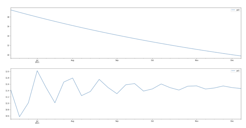
That’s in the case of those two keywords; if you were to try the code on your other data based on more established queries, they will probably provide more accurate forecasts on your own data.

The forecast quality will be dependent on how stable the historic patterns are and will obviously not account for unforeseeable events like COVID-19.

Start Forecasting for SEO

If you weren’t excited by Python’s matplot data visualization tool, fear not! You can export the data and forecasts into Excel, Tableau, or another dashboard front end to make them look nicer.

To export your forecasts:

df_pred = pd.concat([pd.Series(res[1]) for res in oos_results], axis=1)
df_pred.columns = [x + str('_preds') for x in ps_unstacked.columns]
df_pred.to_csv('your_forecast_data.csv')

What we learned here is where forecasting using statistical models is useful or is likely to add value for forecasting, particularly in automated systems like dashboards – i.e., when there’s historical data and not when there is a sudden spike, like PS5.

More Resources:

• 6 SEO Tasks to Automate with Python
• 7 Example Projects to Get Started With Python for SEO
• Advanced Technical SEO: A Complete Guide

Featured image: ImageFlow/Shutterstock