

Chances are, you’ve used one of the more popular tools such as Ahrefs or Semrush to analyze your site’s backlinks.
These tools trawl the web to get a list of sites linking to your website with a domain rating and other data describing the quality of your backlinks.
It’s no secret that backlinks play a big part in Google’s algorithm, so it makes sense as a minimum to understand your own site before comparing it with the competition.
While using tools gives you insight into specific metrics, learning to analyze backlinks on your own gives you more flexibility into what it is you’re measuring and how it’s presented.
And although you could do most of the analysis on a spreadsheet, Python has certain advantages.
Other than the sheer number of rows it can handle, it can also more readily look at the statistical side, such as distributions.
In this column, you’ll find step-by-step instructions on how to visualize basic backlink analysis and customize your reports by considering different link attributes using Python.
Not Taking A Seat
We’re going to pick a small website from the U.K. furniture sector as an example and walk through some basic analysis using Python.
So what is the value of a site’s backlinks for SEO?
At its simplest, I’d say quality and quantity.
Quality is subjective to the expert yet definitive to Google by way of metrics such as authority and content relevance.
We’ll start by evaluating the link quality with the available data before evaluating the quantity.
Time to code.
import re
import time
import random
import pandas as pd
import numpy as np
import datetime
from datetime import timedelta
from plotnine import *
import matplotlib.pyplot as plt
from pandas.api.types import is_string_dtype
from pandas.api.types import is_numeric_dtype
import uritools
pd.set_option('display.max_colwidth', None)
%matplotlib inline

root_domain = 'johnsankey.co.uk'
hostdomain = 'www.johnsankey.co.uk'
hostname = 'johnsankey'
full_domain = 'https://www.johnsankey.co.uk'
target_name = 'John Sankey'
We start by importing the data and cleaning up the column names to make it easier to handle and quicker to type for the later stages.
target_ahrefs_raw = pd.read_csv(
    'data/johnsankey.co.uk-refdomains-subdomains__2022-03-18_15-15-47.csv')
List comprehensions are a powerful and less intensive way to clean up the column names.
target_ahrefs_raw.columns = [col.lower() for col in target_ahrefs_raw.columns]
The list comprehension instructs Python to convert the column name to lower case for each column (‘col’) in the dataframe’s columns.
target_ahrefs_raw.columns = [col.replace(' ','_') for col in target_ahrefs_raw.columns]
target_ahrefs_raw.columns = [col.replace('.','_') for col in target_ahrefs_raw.columns]
target_ahrefs_raw.columns = [col.replace('__','_') for col in target_ahrefs_raw.columns]
target_ahrefs_raw.columns = [col.replace('(','') for col in target_ahrefs_raw.columns]
target_ahrefs_raw.columns = [col.replace(')','') for col in target_ahrefs_raw.columns]
target_ahrefs_raw.columns = [col.replace('%','') for col in target_ahrefs_raw.columns]
Though not strictly necessary, I like having a count column as standard for aggregations and a single value column “project” should I need to group the entire table.
target_ahrefs_raw['rd_count'] = 1
target_ahrefs_raw['project'] = target_name
target_ahrefs_raw
-
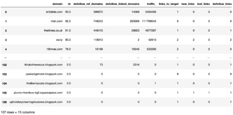
Screenshot from Pandas, March 2022
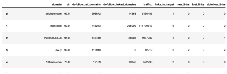
Now we have a dataframe with clean column names.
The next step is to clean the actual table values and make them more useful for analysis.
Make a copy of the previous dataframe and give it a new name.
target_ahrefs_clean_dtypes = target_ahrefs_raw
Clean the dofollow_ref_domains column, which tells us how many ref domains the site linking has.
In this case, we’ll convert the dashes to zeroes and then cast the whole column as a whole number.
# referring_domains
target_ahrefs_clean_dtypes['dofollow_ref_domains'] = np.where(target_ahrefs_clean_dtypes['dofollow_ref_domains'] == '-',
                                                              0, target_ahrefs_clean_dtypes['dofollow_ref_domains'])
target_ahrefs_clean_dtypes['dofollow_ref_domains'] = target_ahrefs_clean_dtypes['dofollow_ref_domains'].astype(int)


# linked_domains
target_ahrefs_clean_dtypes['dofollow_linked_domains'] = np.where(target_ahrefs_clean_dtypes['dofollow_linked_domains'] == '-',
                                                           0, target_ahrefs_clean_dtypes['dofollow_linked_domains'])
target_ahrefs_clean_dtypes['dofollow_linked_domains'] = target_ahrefs_clean_dtypes['dofollow_linked_domains'].astype(int)
First_seen tells us the date the link was first found.
We’ll convert the string to a date format that Python can process and then use this to derive the age of the links later on.
# first_seen
target_ahrefs_clean_dtypes['first_seen'] = pd.to_datetime(target_ahrefs_clean_dtypes['first_seen'], format='%d/%m/%Y %H:%M')
Converting first_seen to a date also means we can perform time aggregations by month and year.
This is useful as it’s not always the case that links for a site will get acquired daily, although it would be nice for my own site if it did!
target_ahrefs_clean_dtypes['month_year'] = target_ahrefs_clean_dtypes['first_seen'].dt.to_period('M')
The link age is calculated by taking today’s date and subtracting the first_seen date.
Then it’s converted to a number format and divided by a huge number to get the number of days.
# link age
target_ahrefs_clean_dtypes['link_age'] = datetime.datetime.now() - target_ahrefs_clean_dtypes['first_seen']
target_ahrefs_clean_dtypes['link_age'] = target_ahrefs_clean_dtypes['link_age']
target_ahrefs_clean_dtypes['link_age'] = target_ahrefs_clean_dtypes['link_age'].astype(int)
target_ahrefs_clean_dtypes['link_age'] = (target_ahrefs_clean_dtypes['link_age']/(3600 * 24 * 1000000000)).round(0)
target_ahrefs_clean_dtypes
With the data types cleaned, and some new data features created, the fun can begin!
Link Quality
The first part of our analysis evaluates link quality, which summarizes the whole dataframe using the describe function to get descriptive statistics of all the columns.
target_ahrefs_analysis = target_ahrefs_clean_dtypes
target_ahrefs_analysis.describe()
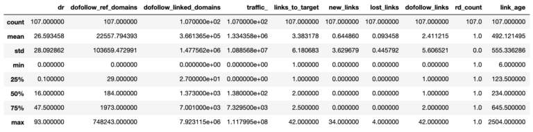
So from the above table, we can see the average (mean), the number of referring domains (107), and the variation (the 25th percentile and so on).
The average Domain Rating (equivalent to Moz’s Domain Authority) of referring domains is 27.
Is that a good thing?
In the absence of competitor data to compare in this market sector, it’s hard to know. This is where your experience as an SEO practitioner comes in.
However, I’m certain we could all agree that it could be higher.
How much higher to make a shift is another question.
The table above can be a bit dry and hard to visualize, so we’ll plot a histogram to get an intuitive understanding of the referring domain’s authority.
dr_dist_plt = (
    ggplot(target_ahrefs_analysis, aes(x = 'dr')) +
    geom_histogram(alpha = 0.6, fill = 'blue', bins = 100) +
    scale_y_continuous() +
    theme(legend_position = 'right'))
dr_dist_plt
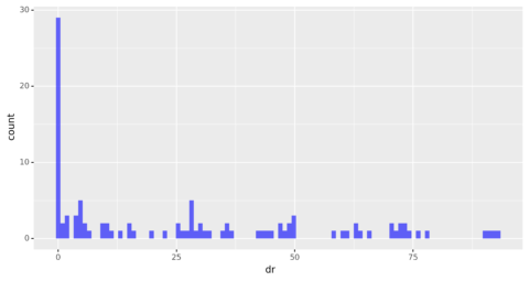
The distribution is heavily skewed, showing that most of the referring domains have an authority rating of zero.
Beyond zero, the distribution looks fairly uniform, with an equal amount of domains across different levels of authority.
Link age is another important factor for SEO.
Let’s check out the distribution below.
linkage_dist_plt = (
    ggplot(target_ahrefs_analysis,
           aes(x = 'link_age')) +
    geom_histogram(alpha = 0.6, fill = 'blue', bins = 100) +
    scale_y_continuous() +
    theme(legend_position = 'right'))
linkage_dist_plt
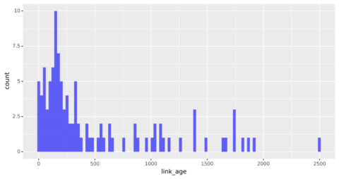
The distribution looks more normal even if it is still skewed with the majority of the links being new.
The most common link age appears to be around 200 days, which is less than a year, suggesting most of the links were acquired recently.
Out of interest, let’s see how this correlates with domain authority.
dr_linkage_plt = (
    ggplot(target_ahrefs_analysis,
           aes(x = 'dr', y = 'link_age')) +
    geom_point(alpha = 0.4, colour = 'blue', size = 2) +
    geom_smooth(method = 'lm', se = False, colour = 'red', size = 3, alpha = 0.4)
)

print(target_ahrefs_analysis['dr'].corr(target_ahrefs_analysis['link_age']))
dr_linkage_plt

0.1941101232345909
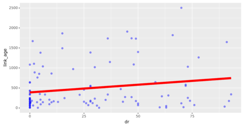
The plot (along with the 0.19 figure printed above) shows no correlation between the two.
And why should there be?
A correlation would only imply that the higher authority links were acquired in the early phase of the site’s history.
The reason for the non-correlation will become more apparent later on.
We’ll now look at the link quality throughout time.
If we were to literally plot the number of links by date, the time series would look rather messy and less useful as shown below (no code supplied to render the chart).
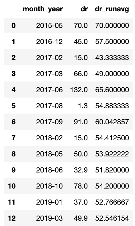
To achieve this, we will calculate a running average of the Domain Rating by month of the year.
Note the expanding( ) function, which instructs Pandas to include all previous rows with each new row.
target_rd_cummean_df = target_ahrefs_analysis
target_rd_mean_df = target_rd_cummean_df.groupby(['month_year'])['dr'].sum().reset_index()
target_rd_mean_df['dr_runavg'] = target_rd_mean_df['dr'].expanding().mean()
target_rd_mean_df
We now have a table that we can use to feed the graph and visualize it.
dr_cummean_smooth_plt = (
    ggplot(target_rd_mean_df, aes(x = 'month_year', y = 'dr_runavg', group = 1)) +
    geom_line(alpha = 0.6, colour = 'blue', size = 2) +
    scale_y_continuous() +
    scale_x_date() +
    theme(legend_position = 'right',
          axis_text_x=element_text(rotation=90, hjust=1)
         ))
dr_cummean_smooth_plt
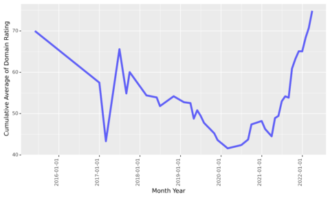
This is quite interesting as it seems the site started off attracting high authority links at the beginning of its time (probably a PR campaign launching the business).
It then faded for four years before reprising with a new link acquisition of high authority links again.
Volume Of Links
It sounds good just writing that heading!
Who wouldn’t want a large volume of (good) links to their site?
Quality is one thing; volume is another, which is what we’ll analyze next.
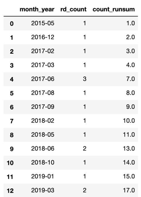
Much like the previous operation, we’ll use the expanding function to calculate a cumulative sum of the links acquired to date.
target_count_cumsum_df = target_ahrefs_analysis
target_count_cumsum_df = target_count_cumsum_df.groupby(['month_year'])['rd_count'].sum().reset_index()
target_count_cumsum_df['count_runsum'] = target_count_cumsum_df['rd_count'].expanding().sum()
target_count_cumsum_df
That’s the data, now the graph.
target_count_cumsum_plt = (
    ggplot(target_count_cumsum_df, aes(x = 'month_year', y = 'count_runsum', group = 1)) +
    geom_line(alpha = 0.6, colour = 'blue', size = 2) +
    scale_y_continuous() +
    scale_x_date() +
    theme(legend_position = 'right',
          axis_text_x=element_text(rotation=90, hjust=1)
         ))
target_count_cumsum_plt
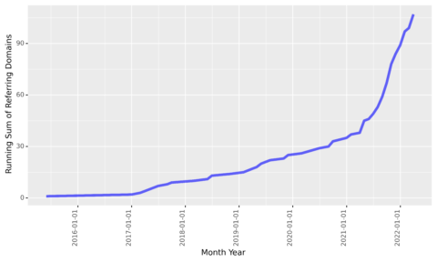
We see that links acquired at the beginning of 2017 slowed down but steadily added over the next four years before accelerating again around March 2021.
Again, it would be good to correlate that with performance.
Taking It Further
Of course, the above is just the tip of the iceberg, as it’s a simple exploration of one site. It’s difficult to infer anything useful for improving rankings in competitive search spaces.
Below are some areas for further data exploration and analysis.
- Adding social media share data to both the destination URLs.
- Correlating overall site visibility with the running average DR over time.
- Plotting the distribution of DR over time.
- Adding search volume data on the host names to see how many brand searches the referring domains receive as a measure of true authority.
- Joining with crawl data to the destination URLs to test for content relevance.
- Link velocity – the rate at which new links from new sites are acquired.
- Integrating all of the above ideas into your analysis to compare to your competitors.
I’m certain there are plenty of ideas not listed above, feel free to share below.
More resources:
- Python SEO Script: Top Keyword Opportunities Within Striking Distance
- An Introduction To Python & Machine Learning For Technical SEO
- Link Building Guide: How to Acquire & Earn Links That Boost Your SEO
Featured Image: metamorworks/Shutterstock
