

My original plan was to cover this topic: “How to Build a Bot to Automate your Mindless Tasks using Python and BigQuery”. I made some slight course changes, but hopefully, the original intention remains the same!
The inspiration for this article comes from this tweet from JR Oakes. 🙂
I think I just have the inspiration I was looking for for my next @sejournal column "How to build a bot to automate your mindless tasks using #python and @bigquery" 🤓 Thanks JR! 🍺 https://t.co/dQqULIH2p2
— Hamlet 🇩🇴 (@hamletbatista) July 12, 2019
As Uber released an updated version of Ludwig and Google also announced the ability to execute Tensorflow models in BigQuery, I thought the timing couldn’t be better.
In this article, we will revisit the intent classification problem I addressed before, but we will replace our original encoder for a state of the art one: BERT, which stands for Bidirectional Encoder Representations from Transformers.
This small change will help us improve the model accuracy from a 0.66 combined test accuracy to 0.89 while using the same dataset and no custom coding!
Here is our plan of action:
- We will rebuild the intent classification model we built on part one, but we will leverage pre-training data using a BERT encoder.
- We will test it again against the questions we pulled from Google Search Console.
- We will upload our queries and intent predictions data to BigQuery.
- We will connect BigQuery to Google Data Studio to group the questions by their intention and extract actionable insights we can use to prioritize content development efforts.
- We will go over the new underlying concepts that help BERT perform significantly better than our previous model.
Setting up Google Colaboratory
As in part one, we will run Ludwig from within Google Colaboratory in order to use their free GPU runtime.
First, run this code to check the Tensorflow version installed.
import tensorflow as tf; print(tf.__version__)
Let’s make sure our notebook uses the right version expected by Ludwig and that it also supports the GPU runtime.
I get 1.14.0 which is great as Ludwig requires at least 1.14.0
Under the Runtime menu item, select Python 3 and GPU.
You can confirm you have a GPU by typing:
! nvidia-smi
At the time of this writing, you need to install some system libraries before installing the latest Ludwig (0.2). I got some errors that they later resolved.
!apt-get install libgmp-dev libmpfr-dev libmpc-dev
When the installation failed for me, I found the solution from this StackOverflow answer, which wasn’t even the accepted one!
!pip install ludwig
You should get:
Successfully installed gmpy-1.17 ludwig-0.2
Prepare the Dataset for Training
We are going to use the same question classification dataset that we used in the first article.
After you log in to Kaggle and download the dataset, you can use the code to load it to a dataframe in Colab.
Configuring the BERT Encoder
Instead of using the parallel CNN encoder that we used in the first part, we will use the BERT encoder that was recently added to Ludwig.
This encoder leverages pre-trained data that enables it to perform better than our previous encoder while requiring far less training data. I will explain how it works in simple terms at the end of this article.
Let’s first download a pretrained language model. We will download the files for the model BERT-Base, Uncased.
I tried the bigger models first, but hit some roadblocks due to their memory requirements and the limitations in Google Colab.
!wget https://storage.googleapis.com/bert_models/2018_10_18/uncased_L-12_H-768_A-12.zip
Unzip it with:
!unzip uncased_L-12_H-768_A-12.zip
The output should look like this:
Archive:  uncased_L-12_H-768_A-12.zip
   creating: uncased_L-12_H-768_A-12/
  inflating: uncased_L-12_H-768_A-12/bert_model.ckpt.meta
  inflating: uncased_L-12_H-768_A-12/bert_model.ckpt.data-00000-of-00001
  inflating: uncased_L-12_H-768_A-12/vocab.txt
  inflating: uncased_L-12_H-768_A-12/bert_model.ckpt.index
  inflating: uncased_L-12_H-768_A-12/bert_config.json
Now we can put together the model definition file.
Let’s compare it to the one we created in part one.
I made a number of changes. Let’s review them.
I essentially changed the encoder from parallel_cnn to bert and added extra parameters required by bert: config_path, checkpoint_path, word_tokenizer, word_vocab_file, padding_symbol, and unknown_symbol.
Most of the values come from the language model we downloaded.
I added a few more parameters that I figured out empirically: batch_size, learning_rate and word_sequence_length_limit.
The default values Ludwig uses for these parameters don’t work for the BERT encoder because they are way off compared to the pre-trained data. I found some working values in the BERT documentation.
The training process is the same as we’ve done previously. However, we need to install bert-tensorflow first.
!pip install bert-tensorflow
!ludwig experiment \

  --data_csv Question_Classification_Dataset.csv\

  --model_definition_file model_definition.yaml
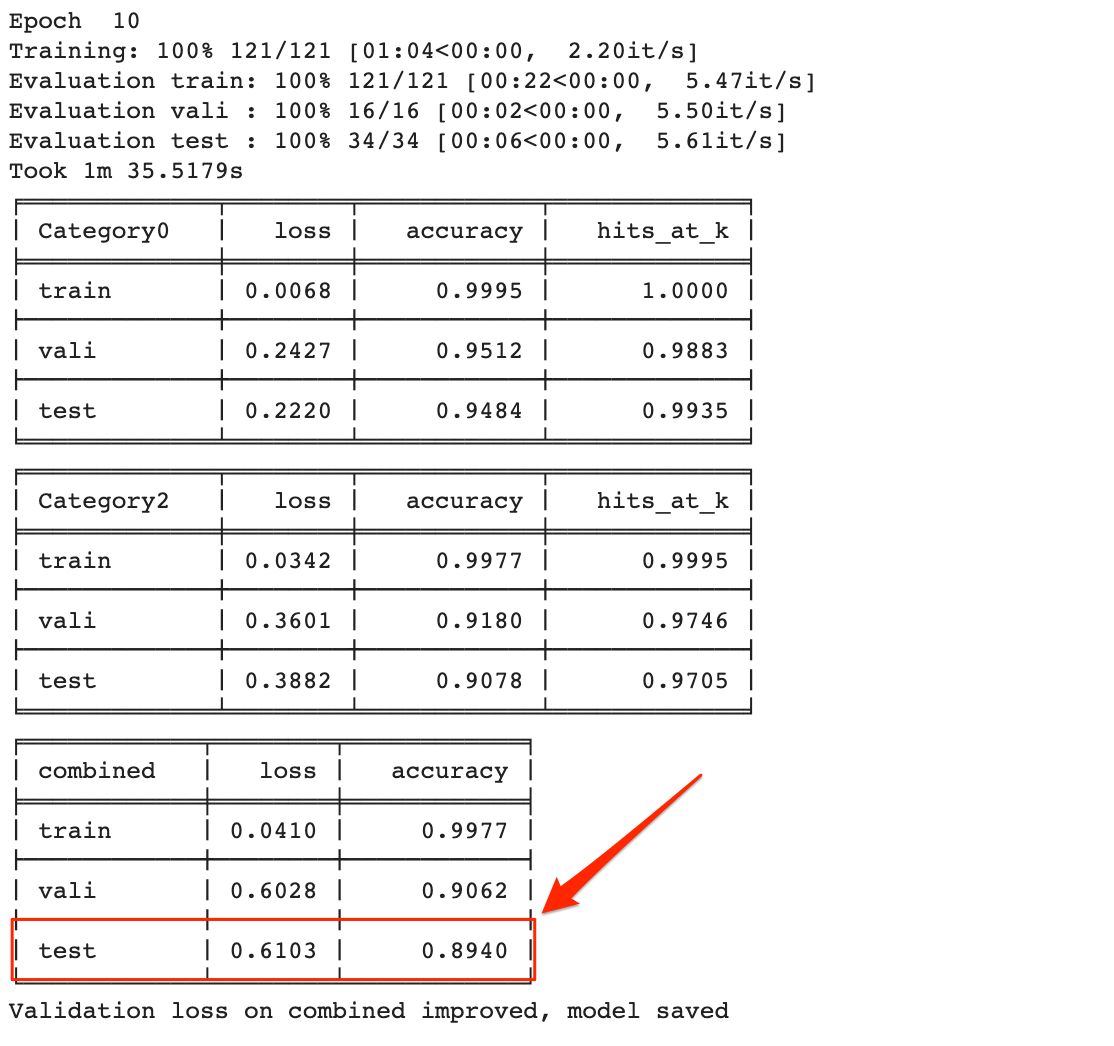
We beat our previous model performance after only two epochs.
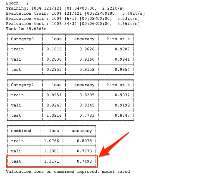
The final improvement was 0.89 combined test accuracy after 10 epochs. Our previous model took 14 epochs to get to .66.
This is pretty remarkable considering we didn’t write any code. We only changed some settings.
It is incredible and exciting how fast deep learning research is improving and how accessible it is now.
Why BERT Performs So Well
There are two primary advantages from using BERT compared to traditional encoders:
- The bidirectional word embeddings.
- The language model leveraged through transfer learning.
Bidirectional Word Embeddings
When I explained word vectors and embeddings in part one, I was referring to the traditional approach (I used a GPS analogy of coordinates in an imaginary space).
Traditional word embedding approaches assign the equivalent of a GPS coordinate to each word.
Let’s review the different meanings of the word “Washington” to illustrate why this could be a problem in some scenarios.
- George Washington (person)
- Washington (State)
- Washington D.C. (City)
- George Washington Bridge (bridge)
The word “Washington” above represents completely different things and a system that assigns the same coordinates regardless of context, won’t be very precise.
If we are in Google’s NYC office and we want to visit “Washington”, we need to provide more context.
- Are we planning to visit the George Washington memorial?
- Do we plan to drive south to visit Washington, D.C.?
- Are we planning a cross country trip to Washington State?
As you can see in the text, the surrounding words provide some context that can more clearly define what “Washington” might mean.
If you read from left to right, the word George, might indicate you are talking about the person, and if you read from right to left, the word D.C., might indicate you are referring to the city.
But, you need to read from left to right and from right to left to tell you actually want to visit the bridge.
BERT works by encoding different word embeddings for each word usage, and relies on the surrounding words to accomplish this. It reads the context words bidirectionally (from left to right and from right to left).
Back to our GPS analogy, imagine an NYC block with two Starbucks coffee shops in the same street. If you want to get to a specific one, it would be much easier to refer to it by the businesses that are before and/or after.
Transfer Learning
Transfer learning is probably one of the most important concepts in deep learning today. It makes many applications practical even when you have very small datasets to train on.
Traditionally, transfer learning was primarily used in computer vision tasks.
You typically have research groups from big companies (Google, Facebook, Stanford, etc.) train an image classification model on a large dataset like that from Imagenet.
This process would take days and generally be very expensive. But, once the training is done, the final part of the trained model is replaced, and retrained on new data to perform similar but new tasks.
This process is called fine tuning and works extremely well. Fine tuning can take hours or minutes depending on the size of the new data and is accessible to most companies.
Let’s get back to our GPS analogy to understand this.
Say you want to travel from New York City to Washington state and someone you know is going to Michigan.
Instead of renting a car to go all the way, you could hike that ride, get to Michigan, and then rent a car to drive from Michigan to Washington state, at a much lower cost and driving time.
BERT is one of the first models to successful apply transfer learning in NLP (Natural Language Processing). There are several pre-trained models that typically take days to train, but you can fine tune in hours or even minutes if you use Google Cloud TPUs.
Automating Intent Insights with BigQuery & Data Studio
Now that we have a trained model, we can test on new questions we can grab from Google Search Console using the report I created on part one.
We can run the same code as before to generate the predictions.
This time, I also want to export them to a CSV and import into BigQuery.
test_df.join(predictions)[["Query", "Clicks", "Impressions", "Category0_predictions", "Category2_predictions"]].to_csv("intent_predictions.csv")
First, log in to Google Cloud.
!gcloud auth login --no-launch-browser
Open the authorization window in a separate tab and copy the token back to Colab.
Create a bucket in Google Cloud Storage and copy the CSV file there. I named my bucket bert_intent_questions.
This command will upload our CSV file to our bucket.
!gsutil cp -r intent_predictions.csv gs://bert_intent_questions
You should also create a dataset in BigQuery to import the file. I named my dataset bert_intent_questions
!bq load --autodetect --source_format=CSV bert_intent_questions.intent_predictions gs://bert_intent_questions/intent_predictions.csv
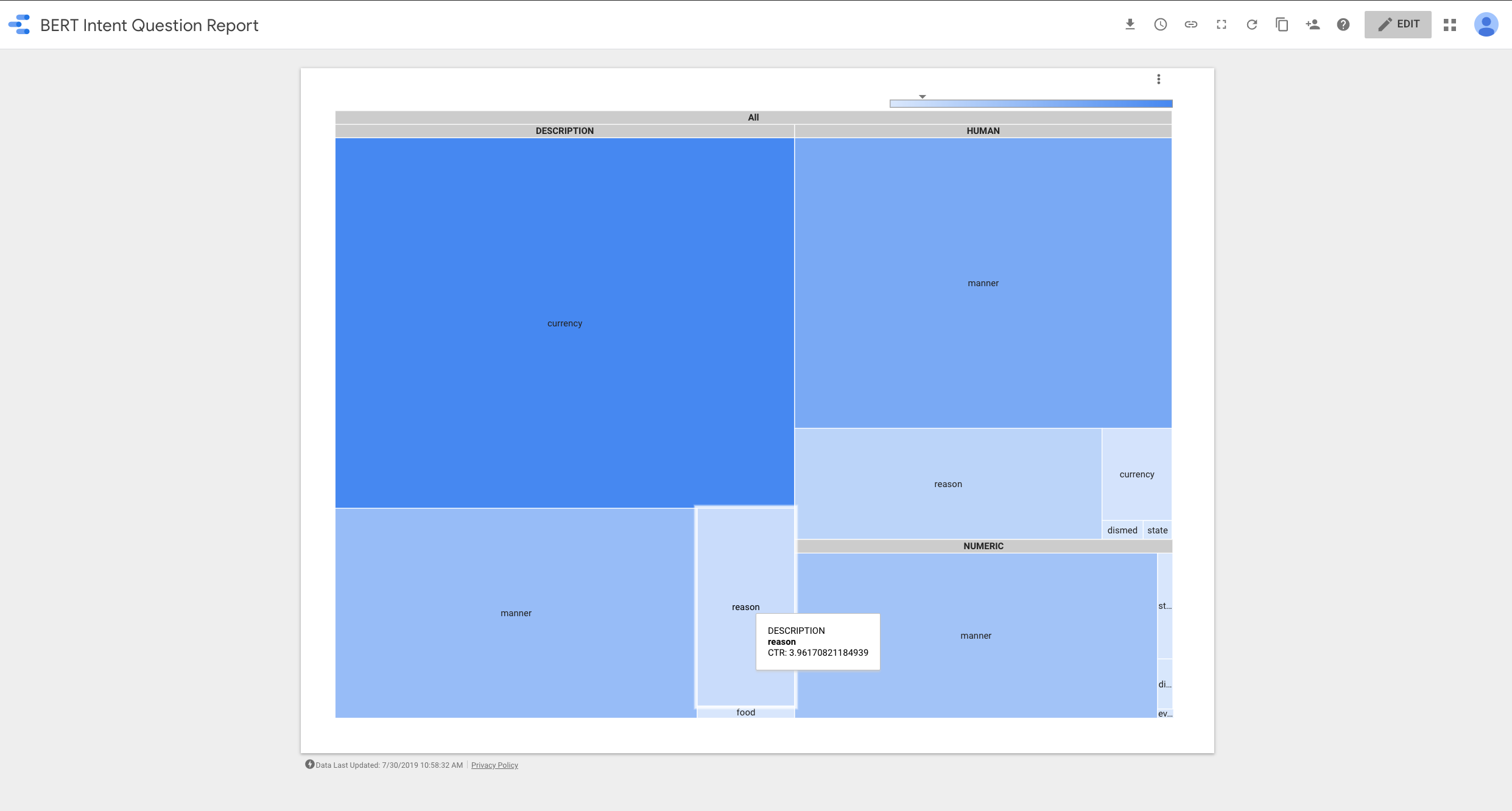
After we have our predictions in BigQuery, we can connect it to Data Studio and create a super valuable report to helps us visualize which intentions have the greatest opportunity.
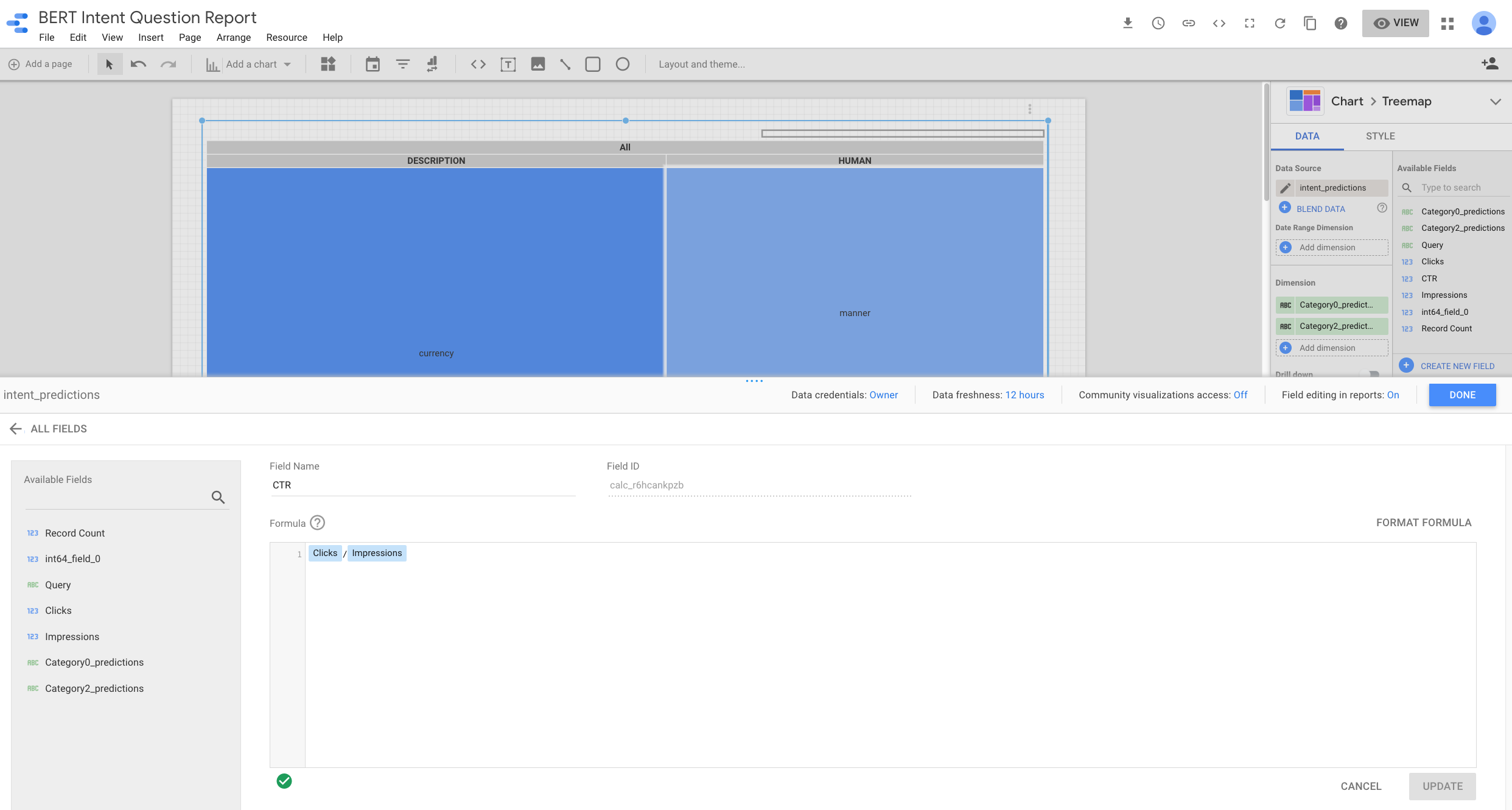
After I connected Data Studio to our BigQuery dataset, I created a new field: CTR by dividing impressions and clicks.
As we are grouping queries by their predicted intentions, we can find content opportunities where we have intentions with high search impressions and low number of clicks. Those are the lighter blue squares.
How the Learning Process Works
I want to cover this last foundational topic to expand the encoder/decoder idea I briefly covered in part one.
Let’s take a look at the charts below that help us visualize the training process.
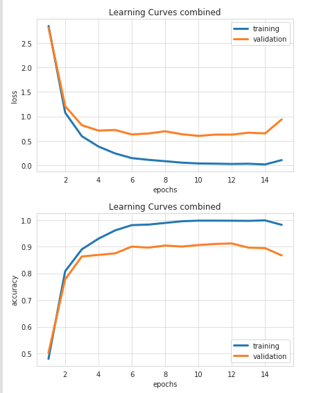
But, what exactly is happening here? How it the machine learning model able to perform the tasks we are training on?
The first chart shows how the error/loss decreases which each training steps (blue line).
But, more importantly, the error also decreases when the model is tested on “unseen” data. Then, comes a point where no further improvements take place.
I like to think about this training process as removing noise/errors from the input by trial and error, until you are left with what is essential for the task at hand.
There is some random searching involved to learn what to remove and what to keep, but as the ideal output/behavior is known, the random search can be super selective and efficient.
Let’s say again that you want to drive from NYC to Washington and all the roads are covered with snow. The encoder, in this case, would play the role of a snowblower truck with the task of carving out a road for you.
It has the GPS coordinates of the destination and can use it to tell how far or close it is, but needs to figure out how to get there by intelligent trial and error. The decoder would be our car following the roads created by the snowblower for this trip.
If the snowblower moves too far south, it can tell it is going in the wrong direction because it is getting farther from the final GPS destination.
A Note on Overfitting
After the snowblower is done, it is tempting to just memorize all the turns required to get there, but that would make our trip inflexible in the case we need to take detours and have no roads carved out for that.
So, memorizing is not good and is called overfitting in deep learning terms. Ideally, the snowblower would carve out more than one way to get to our destination.
In other words, we need as generalized routes as possible.
We accomplish this by holding out data during the training process.
We use testing and validation datasets to keep our models as generic as possible.
A Note on Tensorflow for BigQuery
I tried to run our predictions directly from BigQuery, but hit a roadblock when I tried to import our trained model.
!bq query \
--use_legacy_sql=false \
"CREATE MODEL \
bert_intent_questions.BERT \
OPTIONS \
(MODEL_TYPE='TENSORFLOW', \
MODEL_PATH='gs://bert_intent_questions/*')" \
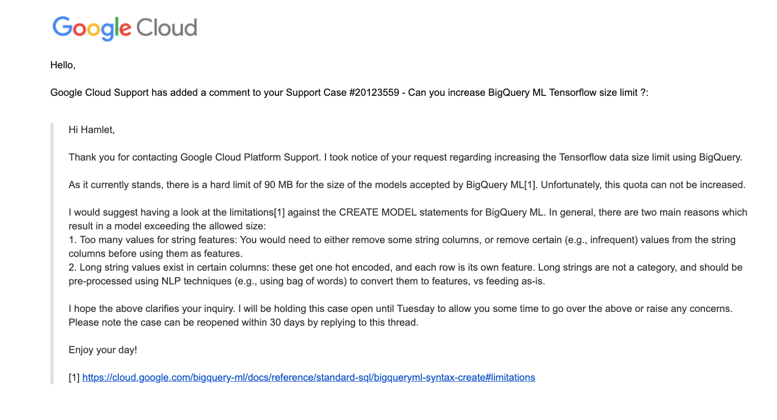
BigQuery complained about the size of the model exceeded their limit.
Waiting on bqjob_r594b9ea2b1b7fe62_0000016c34e8b072_1 ... (0s) Current status: DONE BigQuery error in query operation: Error processing job 'sturdy-now-248018:bqjob_r594b9ea2b1b7fe62_0000016c34e8b072_1': Error while reading data, error message: Total TensorFlow data size exceeds max allowed size; Total size is at least: 1319235047; Max allowed size is: 268435456
I reached out to their support and they offered some suggestions. I’m sharing them here in case someone finds the time to test them out.
Resources to Learn More
When I started taking deep learning classes, I didn’t see BERT or any of the latest state of the art neural network architectures.
However, the foundation I received, has helped me pick up new concepts and ideas fairly quickly. One of the articles that I found most useful to learn the new advances was this one: The Illustrated BERT, ELMo, and co. (How NLP Cracked Transfer Learning).
I also found this one very useful: Paper Dissected: BERT: Pre-training of Deep Bidirectional Transformers for Language Understanding” Explained and this other one from the same publication: Paper Dissected: “XLNet: Generalized Autoregressive Pretraining for Language Understanding” Explained.
BERT has recently been beaten by a new model called XLNet. I am hoping to cover it in a future article when it becomes available in Ludwig.
The Python momentum in the SEO community continues to grow. Here are some examples:
Paul Shapiro brought Python to the MozCon stage earlier this month. He shared the scripts he discussed during his talk.
I was pleasantly surprised when I shared a code snippet in Twitter and Tyler Reardon, a fellow SEO, quickly spotted a bug I missed because he created a similar code independently.
Big shoutout to @TylerReardon who spotted a bug in my code pretty quickly! It is already fixed https://t.co/gvypIOVuBp
I thought I was comparing the IP from the log and the one from the DNS, but I was comparing the log IP twice! 😅
We have an awesome #python #SEO community 💪
— Hamlet 🇩🇴 (@hamletbatista) July 25, 2019
Michael Weber shared his awesome ranking predictor that uses a multi-layer perceptron classifier and Antoine Eripret shared a super valuable robot.txt change monitor!
I should also mention that JR contributed a very useful Python piece for opensource.com that shows practical uses cases of the Google Natural Language API.
More Resources:
- Automated Intent Classification Using Deep Learning
- Advanced Duplicate Content Consolidation with Python
- Advanced Technical SEO: A Complete Guide
Image Credits
All screenshots taken by author, July 2019
